A quantitative schedule risk analysis (QSRA) usually ends with a P80 date and a tornado chart. Both answer the question the client asks, and neither explains the latest finishes, where a contractor loses money, or the combinations of risks behind them. This post is for planners who already run QSRA and want more from the result: how to read its shape, why the worst outcomes come from risks landing together, and how Planlab's AI agent explains that for you.
I work on Planlab's risk analysis tools. When our team spent a day working through QSRA results with a contractor's planners, nobody asked about the P80. They asked what has to go wrong for the job to end up in the bad part of the chart, and whether they could stop it. The standard outputs do not answer that, and I think they should.
A QSRA result is thousands of possible projects, not one date
QSRA software replays the schedule thousands of times. In each run, every activity draws a duration from its uncertainty range and every risk in the register either happens or does not. The critical path is recalculated each time, so the output is one finish date per run. The S-curve and the P-dates are summaries of those runs.
Read the shape before you quote a number. On the S-curve, a steep section means many runs finish close together. A shallow section means runs are spread thinly over many weeks. A curve that climbs steeply and then crawls for months has a long tail.
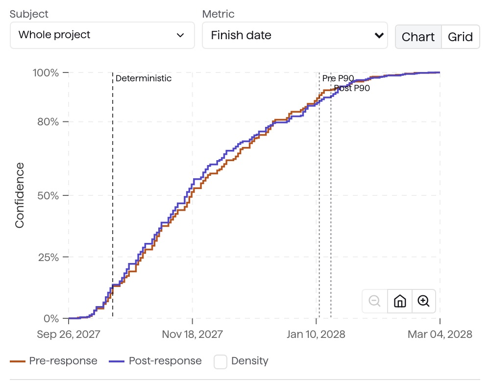
The S-curve for Tarrow Mill, a fictional demonstration footbridge project. The dashed line on the left is the planned finish. The last tenth of the runs spreads over two months.
The fat tail is where a contractor's margin goes
A fat tail is the part of a risk analysis result where a meaningful share of runs finish far later than the rest, rather than a few outliers. Construction results tend to have one, because there are few ways to finish much earlier than planned and many ways to finish much later.
Longer delays cost more, and the tail holds the longest. Site staff, plant, welfare and insurance keep running while the work runs late, and once the job passes its completion date, as adjusted for any extensions, delay damages apply on top. The runs in the tail are where both add up, so they decide whether the job makes its margin.
The demonstration project in this post has a contractual handover of 15 October 2027. Its QSRA gives it about a 13% chance of making that date, and its P90 lands 89 days after it.
A tornado chart ranks risks one at a time; overruns come from combinations
To build a tornado chart, the software removes one risk at a time and measures how much the result improves. That answers "which single risk matters most?" It cannot show the pattern behind most bad outcomes on site: one thing going wrong is survivable, and two or three together push the job into a much worse state.
At Tarrow Mill, runs with a late possession alone finished a median 55 days late; with a welder shortage as well, 91. Both are calendar days past the contract date. Every run in the worst 10% includes the late site possession, and most include a second risk as well:
| Risks that happened | Share of the worst 10% | Median days late, all runs with these risks |
|---|---|---|
| Late possession + welder shortage | 36% | 91 |
| Late possession + piling vibration limits | 14% | 77 |
| Late possession + welder shortage + approval redesign | 14% | 111 |
| Late possession + approval redesign + piling limits | 11% | 103 |
| Other combinations with late possession | 25% | 84 to 139 |
Each tornado bar is one risk removed. In Planlab's QSRA panel, a bar shows how far the P90 moves when that one risk is taken out and every other risk stays in. On the Tarrow Mill simulation, the five single-risk bars add up to about 46 working days, while removing all five threats together moves the P90 about 57. P-date changes do not add, so the bars cannot tell you which risks combine. The combination table above can.
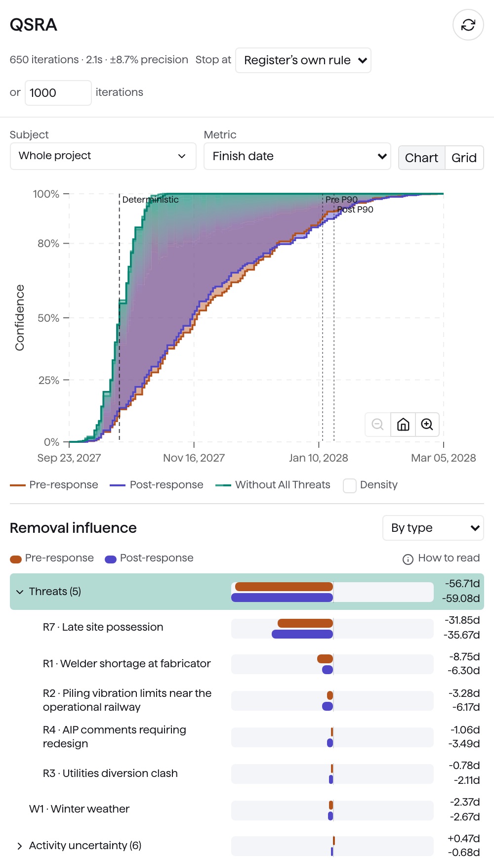
The tornado for the fictional Tarrow Mill demonstration project, in working days, with the threats expanded and the all-threats curve overlaid.
Group the worst runs by the risks that happened in them
Planlab's AI agent does this grouping for you. After a run it looks at the shape of the distribution and picks the part the team cares about: the P90 tail by default, or the percentile your bid uses. Then it groups the runs by which risks happened in them and says which combinations put a run in the tail.
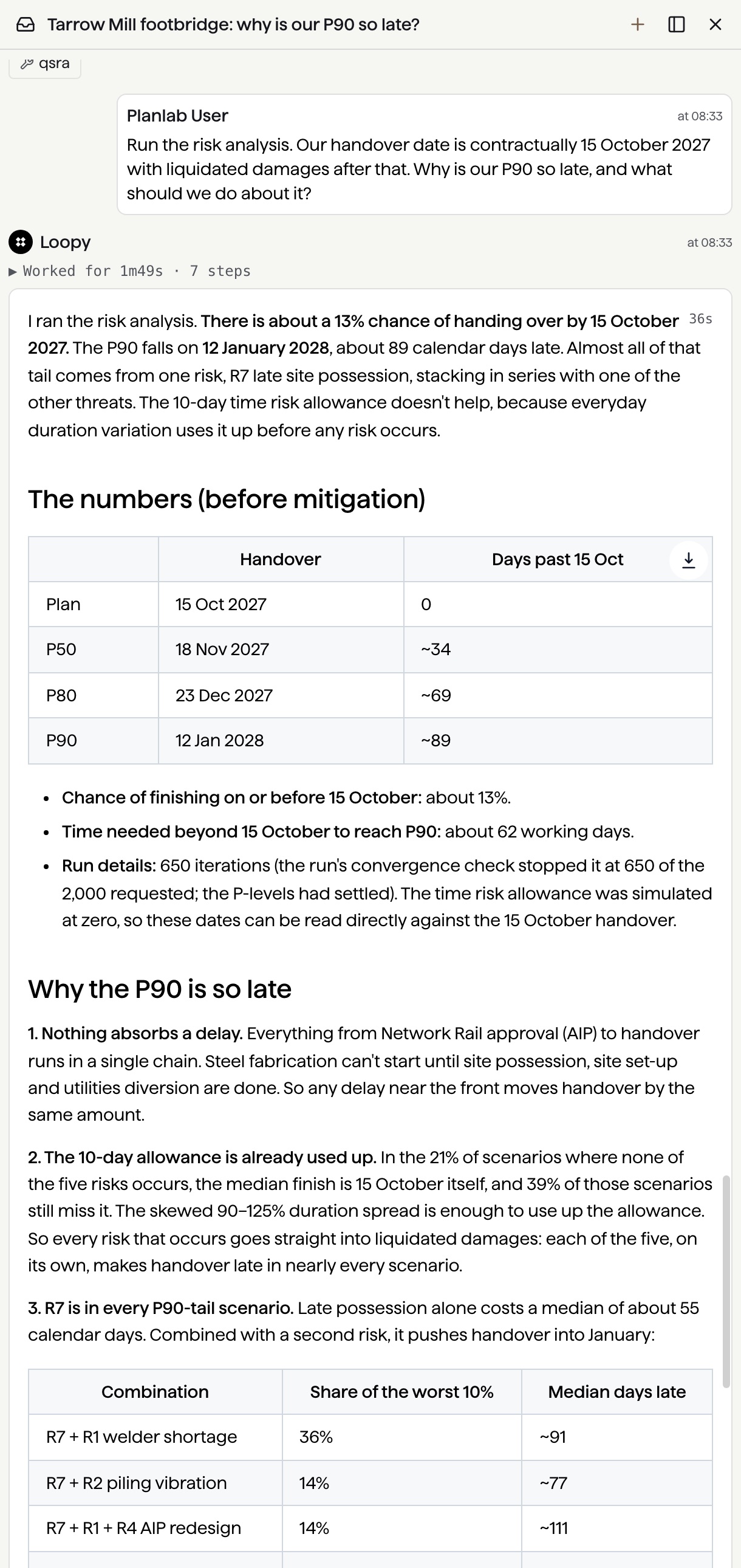
The agent's answer on the fictional Tarrow Mill demonstration project, asked why the P90 is so late.
The useful answer is often a change to the schedule logic. At Tarrow Mill, the agent pointed out that steel fabrication, which happens off site, was tied to site possession in the logic. It estimated, without re-running the simulation, that starting fabrication after design approval would give it about 20 days of float, absorb most of the welder shortage, and separate the two risks that fill most of the tail. It also noted that under the NEC4 Engineering and Construction Contract, failing to give access by the access date is a compensation event, which can move the Completion Date, subject to assessment.
A result with two humps describes two different projects
A bimodal result is a distribution with two separate peaks. It usually comes from one large yes-or-no event: planning consent refused, a possession or outage window missed, a design approval sent back. When the event happens, the whole project shifts by a large step.
The average of a bimodal result describes no real outcome. The mean can fall between the peaks, where few runs land, and a P-date near the edge of a hump can jump by the whole step when the risk's probability moves a few points. State it as two outcomes instead. For example: "if consent is granted, we finish around this date; there is a 35% chance it is refused, and then we finish around that one." Each outcome then gets its own plan and contingency.
Check that your buffers sit where the risk is
Check whether an allowance covers both everyday variation and the risks. Most programmes carry buffers: a time risk allowance activity, float held before a milestone, weather allowances in the calendar. Before simulating, a buffer activity has to be taken out of the simulation, or it double-counts the risk it exists to absorb. After simulating, the largest buffer should protect the path that the tail's risks hit.
At Tarrow Mill, the agent found the 10-day time risk allowance before simulating and set its duration to zero for the run. In runs where none of the five risks happened, the median finish was the contract date itself and 39% still missed it, so everyday duration variation alone uses up the allowance.
What to take into your next risk review
- Look at the shape first: tight, fat-tailed or bimodal.
- Decide which part of the distribution costs you money.
- Ask which combinations of risks fill that part, not which single risk tops the tornado.
- Report a bimodal result as two outcomes with their chances.
- Check that your buffers protect the paths the tail's risks hit.
The Tarrow Mill simulation assumes a register where risks are independent of each other. On real projects they rarely are: a late possession pushes work into winter, and winter makes welding slower. The next post covers how to model those links. For how the agent builds and updates the register in the first place, see AI QSRA: your risk analyst has joined the project. For keeping the assumptions behind it traceable, see why your project needs a knowledge base.